|
|
Your source of photonics CAD tools | |
|
| ||
FIMMPROPA bi-directional optical propagation tool |
   |
Fiber Bragg Gratings (FBGs)3D simulation of transmission and reflection spectra with FIMMPROP softwareWe will show here how FIMMPROP can be used to model fiber Bragg gratings. We will study three different geometries, and use FIMMPROP to generate transmission and reflection spectra in each case for different mode orders.
FIMMPROP is a very efficient tool for the modelling of optical fiber devices. It can take advantage of the two fully vectorial fiber solvers available in FIMMWAVE and can model continuously varying optical fiber devices, such as sinusoidal fiber Bragg gratings and fiber tapers, as well as discontinuous optical fiber devices such as discrete fiber Bragg gratings, coupling between e.g. a fiber and a planar waveguide and cylindrical MMI couplers. In this example, FIMMPROP was used to model various first-order (lossless) fiber Bragg gratings. FIMMPROP can model such devices very efficiently and accurately:
Geometry of the Fiber Bragg GratingsThe different cross-sections used in the three FBGs are shown below. We used FIMMWAVE's fiber waveguide editor to create the cross-sections for the first two fiber Bragg gratings which are cylindrical, and the mixed geometry waveguide editor to create the cross-sections in the third case where the cylindrical symmetry is broken.
We used the FDM Fibre Solver to calculate the modes for the cylindrically symmetric designs A and B and the FDM Solver for the non-cylindrically symmetric design C. The FDM Fibre Solver uses the well-known finite-difference method to solve the vectorial wave equation in cylindrical co-ordinates, and the FDM Solver uses the same method in Cartesian co-ordinates. These solvers are particularly well suited for this problem:
The number of modes and spatial resolution used by the mode solvers were optimised by performing convergence tests. As FIMMPROP is a frequency-domain tool, the wavelength was varied using the FIMMPROP Scanner, an automated tool allowing to perform parametric scans. The scanner was used to calculate the transmission and reflection spectra into various mode orders. Fiber Bragg Grating A - step index fibreIn this first structure, the period of the grating is made with two sections of step-index fibers with a core and a cladding.
The parameters are given below.
The structure designed in FIMMPROP is shown below, as well as the modes of the fibre. This structure was solved in cylindrical co-ordinates using the FDM Fibre Solver. The simulation was extremely fast; it only took 6.5s for FIMMPROP to generate the scattering matrix for each wavelength, for a device with 20000 periods!
The grating includes 20000 periods. FIMMPROP's power normalise feature was used in the overlaps of the period to compensate for small numerical errors and prevent them from accumulating along the grating. You can see below the transmission spectrum obtained with the FIMMPROP Scanner. As could be expected, only one peak is found at the Bragg wavelength of 1.4849um, where 75% of the light gets reflected.
You can see below the evolution of the transmission spectrum when the numbers of periods is varied; a much smaller scale is used to show the detail of the peak.
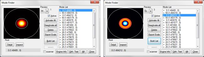
Fiber Bragg Grating B - step index fibre with secondary coreIn this second structure, one of the sections of the grating includes a secondary core. The structure and parameters are shown below. This structure was solved in cylindrical co-ordinates using the FDM Fibre Solver.
In this case, above 50% of the light is reflected in the HE11 mode at 1.4849um, and about 30% of the light gets reflected into the HE21 mode for a slightly lower wavelength of 1.4846um. This simulation took slightly longer as further modes were needed, with a calculation time of 19s for each wavelength - still very fast!
Fiber Bragg Grating C - asymmetric fibreIn this third structure, the core of one of the high-index section of the grating is modified as shown in the diagram. This structure was solved in Cartesian co-ordinates using the FDM Solver.
In this case, 40% of the light is reflected in the HE11 mode at 1.4849um, and about 20% of the light gets reflected into the HE21 mode for a slightly lower wavelength of 1.4846um. This simulation only took 21s for each wavelength.
|
 © 2023 Photon Design copyright all rights reserved |

 |